Introduction
In this project, factors affecting housing prices in the UK context have been studied from 1978 to 2015. The housing market is one of the significant sectors which affect the UK economy. More specifically, housing price inflation in the UK is particularly substantial, which affects the economic aspects of the UK. HM Treasury, in reference to the Barker Report, HM Treasury has described increasing housing prices will have unhelpful and unwelcome consequences for the economic well-being of the UK. The report of PwC (PricewaterhouseCoopers), the world’s second-largest professional services network headquartered in London, states that if current market demand and supply for houses continue, by 2025, more than 50% of the people aged between 20 and 29 years of age will start renting privately (PwC, 2017). Housing prices get affected by many factors, including interest rate, number of houses built per year, and other demand and supply factors (Attanasio and Weber, 2014).
However, the study of housing prices and factors affecting this variable was fascinating because, in reference to the PwC report, I also lie in the age bracket of 20 and 29 years. So, the issue of rising housing prices is also a concern for me from a homeownership perspective. Apart from this motivation, empirical studies on housing prices also showed the importance of its research, where several factors have been identified to affect housing prices (Attanasio and Weber, 2014; Cheng and Fung, 2015). Based on empirical studies, significant elements of housing prices for the 1978-2015 periods have been analysed in the UK context in this project. This project has considered several demand and supply variables and tested four main hypotheses. The hypotheses are:
H1: GDP Per Capita has a positive association with Housing Price.
H2: Houses Built Per Year has a negative association with Housing Price.
H3: Interest Rate has a negative association with Housing Price.
H4: Unemployment Rate has a negative association with Housing Price.
Housing price is also significant from an economic perspective because several factors get involved in the behaviour of housing prices (Cohen and Karpavičiūtė, 2017). The study of Meese and Wallace (2014) argued that interest rate is one of the significant factors that affect housing prices. Increasing interest rates during the inflationary period have been associated with rising housing prices, while it was not valid during the deflationary period that lowering interest rates has no impact on decreasing housing prices (Meese and Wallace, 2014). Gross Domestic Product (GDP) per capita and its association with housing prices have been argued to be positive (Yun Joe Wong, Man Eddie Hui, and Seabrooke, 2013). Fiva and Kirkebøen (2011) argued that higher national income represents the higher ability of people to buy houses, and for this reason, higher GDP may aid in higher housing prices. The number of homes built per year in the UK may be a significant factor as supply in tandem with demand may also help in a hike/decrease in housing prices (Bełej and Kulesza, 2014). Employment within an economy is also an essential determinant of housing prices because a higher unemployment rate means a more significant number of people cannot buy new houses (Cheng and Fung, 2015).
Data Description
This project has studied housing prices and several other variables as its determinants. In order to serve this purpose, this project has used secondary data from archived sources of the UK Government as national-level statistics were essential. Collection of primary data on housing prices, interest rate, number of houses built per year, GDP per capita, and the unemployment rate would have been irrelevant for this project. For instance, housing prices could not be accurately estimated if they were collected primarily through surveys. All these variables have been expressed quarterly between 1978 and 2015. As all these data were collected from UK Government sources, therefore this project did not require any ethical approval. However, the following table provides a brief description of variables:
Table 1: Definition of Variables
Name of Variable | Definition |
Real Housing Price (RHP) | Average housing price in a given year adjusted for inflation (£) |
GDP Per Capita (GDPPC) | Real GDP per capita (£) |
Houses Built Per Year (HBPY) | The aggregate number of houses built per year in the UK |
Interest Rate (IR) | Rate of interest according to the Bank of England (BoE) |
Unemployment Rate (UR) | Rate of unemployed population in the UK |
Real Housing Price
Data on real Housing Prices have been collected from Nationwide society through Halifax, Office for National Statistics (ONS), and Rightmove also provides housing prices data. Nationwide has been chosen over other sources for two reasons. Firstly, Nationwide is the only source that provides the most comprehensive time-series data, extending to 1975. It allowed this project to include more statistical observations in the analysis, which, on the other hand, increased reliability. Secondly, housing price data provided by Nationwide were adjusted for retail price inflation. Inflation-adjusted housing prices provided this project more representative analysis of the issue. For this project, quarterly housing price data has been collected Nationwide.
GDP Per Capita
GDP per capita data on the UK has been collected from the ONS because this dataset was compiled through three GDP measurement approaches: income, output, and expenditure. In the ONS database for GDP, there are three separate estimations for this variable for each quarter which ensures accurate measurement of data. ONS’ database for GDP also adjusts inflation which makes the data more reliable and aids in more representative analysis. Quarterly data on GDP per capita has been collected from ONS’ UK financial accounts.
Houses Built Per Year
Houses built per year data has been collected from the archives of the UK Government. The library includes data on the number of permanent dwellings completed per year, which incorporates properties built by local authorities, housing associations, and the private sector. Quarterly information on houses built per year has been extracted from the UK Government archive and being a government archive, this data must be reliable.
Interest Rate
The online source of the Bank of England (BoE) has been used to obtain interest rate time series data. The time-series data on interest rate is provided both in quarterly and annualised form for each calendar year. This project has chosen quarterly interest rate data. As this data has been collected from the BoE, which sets interest rates, this data should be highly reliable.
Unemployment Rate
Unemployment data has been sourced from the database of ONS. The ONS database for unemployment data excludes economically inactive people (for example, sick, students, retirees, disabled, and people less than 16 years of age). Quarterly data on the unemployment rate has been extracted from the ONS database.
Methods
This project has used several statistical data analysis procedures to study housing prices and their determinants. EViews have been used to analyse this project because this software package allows effective and easier ways of analysing time-series data. First of all, correlations among the variables have been tested. Secondly, this project has tested the time series data stationarity by applying the unit root test. Thirdly, this project has tested for autocorrelation by using the ARMA model in EViews. Fourthly, the Breusch-Pagan-Godfrey test for heteroskedasticity has been carried out. Finally, after adjusting for stationarity, autocorrelation, and heteroskedasticity, ordinary least squares regression has been carried out for final outcomes.
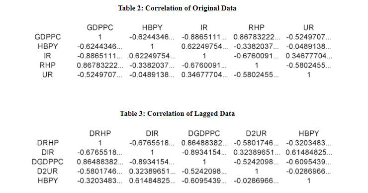
Correlation among all the variables has been calculated based on the data collected from stated sources. Correlation has been carried out to provide information on the nature of associations and the strength of associations among the variables. This helped to understand the characteristic of the relationship between the variables.
Time series data may suffer from non-stationarity because it is possible that variables may be correlated with time. That is, a variable may change over time. Non-stationarity in time series data may indicate a systematic pattern that is unpredictable. Therefore, it was essential to run a unit root test to confirm there is no recurring pattern in the dataset that is unpredictable and affects the outcomes of the analysis.
Ordinary Least Squares (OLS) regression has been carried out for the time-series data, which helped to estimate unknown parameters in the linear regression model. The goal of applying OLS was to minimise the sum of the squares of the differences between observed responses and those predicted by the linear function of a set of explanatory variables. The consistency of OLS estimators is confirmed when regressors are optimal in the class of linear unbiased estimators and exogenous, especially when the errors are serially uncorrelated and homoscedastic.
OLS required a serially uncorrelated and homoscedastic dataset for further data analysis. Therefore, it was also essential to test for serial correlation (autocorrelation) and heteroskedasticity. This project has used the Breusch-Godfrey LM and Durbin-Watson test to examine if the time series data of this project was autocorrelated. To remove autocorrelation from the regression model, this project has used the ARMA (Autoregressive and Moving,-average) model. This project has used the Breusch-Pagan-Godfrey test for heteroskedasticity, which is actually performed to estimate if the variability of a variable is unequal across the range of values of a second variable that predicts it.
However, the OLS equation of this project is:
LOG(RHP(-1)) = C(1) + C(2)*LOG(GDPPC(-1)) + C(3)*LOG(HBPY) + C(4)*LOG(IR(-1)) + C(5)*LOG(UR(-2)) + C(6)*@TREND
In this OLS model;
Log(RHP(-1))= Log the value of First Lag of Real Housing Price
C(1)= Constant of the OLS Regression
C(2)= Coefficient of First Lag of GDP Per Capita
GDPPC(-1)= Log the value of First Lag of GDP Per Capita
C(3)= Coefficient of Houses Built Per Year
Log(HBPY)= Log value of Houses Built Per Year
C(4)= Coefficient of First Lag of Interest Rate
Log(IR(-1))= Log the value of First Lag of Interest Rate
C(5)= Coefficient of Unemployment Rate
Log(UR(-2))= Log value of Second Lag of Unemployment Rate
C(6)= Coefficient of Trend
@Trend= Trend adjustment value for the OLS Model
This OLS model helped to analyse the variables without any error as this project has removed non-stationarity, autocorrelation, and heteroskedasticity within the dataset alongside adjustment for lagged value and trend effect.
Results
Simple Time Series Regression
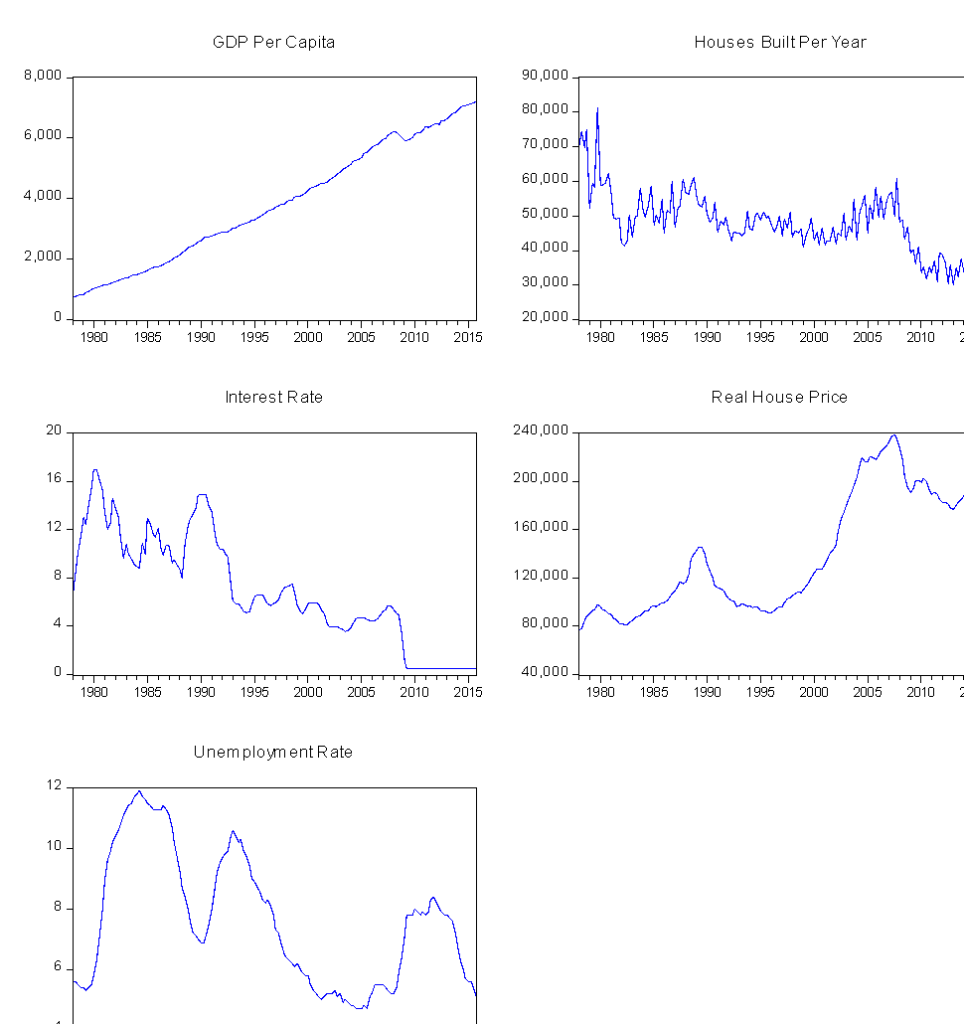
First of all, this project estimated a model that captured movements in housing prices based on GDP per capita, houses built per year, interest rate, and unemployment rate. From the graph presented below, it can be observed that except for GDP Per Capita, other variables have substantial variation across the period surveyed, which may be an indicator of non-stationarity.

However, this project has run simple time-series regression on the raw data, which returned the following output:
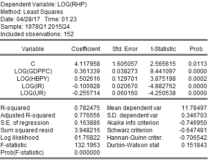
From this simple time-series regression, it can be observed that 78.24% of variations in housing prices have been explained by the variations in the dependent variables (i.e., GDP per capita, houses built per year, interest rate, and unemployment rate). All the variables were statistically significant, with GDP per capita, interest rate, and unemployment rate having an expected sign and houses built per year with an unexpected gesture. From this regression, housing prices get significantly affected by all the variables. As it has been said earlier that time-series data may change along with time, i.e., it may not be stationary. For this reason, a unit root test has been carried out to see if the dataset is stationary.
The unit root test for all the variables indicated that only houses built per year were stationary while all other variables were non-stationary. The unit root test for real housing price indicated that RHP was non-stationary at a level while it was stationary at its first difference or lag. Similarly, GDPPC and IR were also non-stationary at their level and stationary at their first lag. UR was non-stationary at the level and its first lag but was stationary at its second difference. HBPY was stationary at its level. Therefore, for further econometric analysis, this project has used the first lag of RHP, GDPPC, and IR, the second lag of UR, and the level data of HBPY. Results of the unit root test are provided in Appendix. However, after correcting data from non-stationary to stationary, the least-squares regression provided the following output:

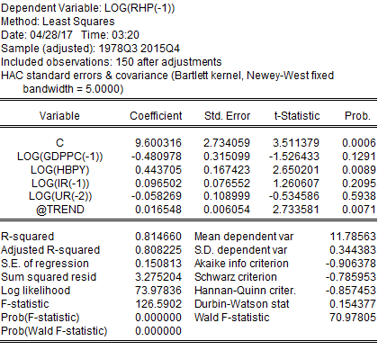
Similar to the earlier regression, current regression also provides similar results, although it has been adjusted for non-stationarity. As the results did not vary substantially, this project considers adjusting for trends because economic time series data has a tendency to grow over time. Therefore, ignoring the fact of time trend can lead this project to falsely conclude regarding the impact of one variable on the other. Finding the relationship between two or more trending variables was essential because they grow over time, indicating a spurious regression problem. For this reason, this project has added a time trend to this regression model. After adjusting for the time trend following result is found:
From the time trend adjusted regression output, it can be seen that IR and UR became statistically insignificant, and IR lost its expected sign. Furthermore, in the previous regression coefficient of GDPPC was positive and statistically significant, but this regression indicates that it has a negative coefficient and it is statistically insignificant.
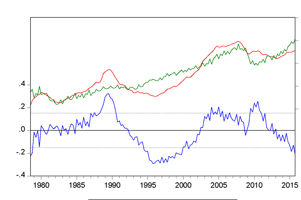
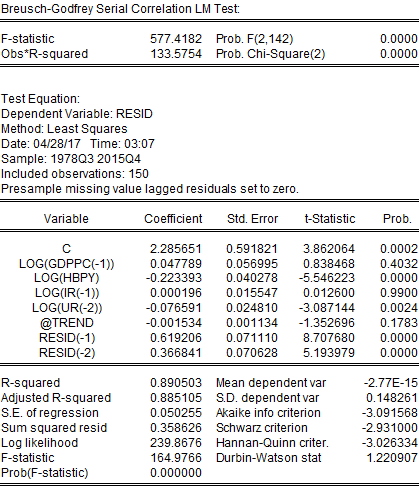
The above figure is the actual, fitted, and residual plot of this regression, where the behaviour of residuals appears to be correlated with their own lagged values, which indicate serial correlation. Serial correlation is very common in time-series data as data remains in ordered form over time. OLS regression assumes that error terms are uncorrelated, and it is violated in the above regression where error terms seem to be correlated. It was important to treat serial correlation because in the presence of lagged dependent variables, the estimates provided by OLS will be inconsistent and biased. For this reason, this project has tested for serial correlation by using Durbin-Watson statistics and the Breusch-Godfrey test for serial correlation.
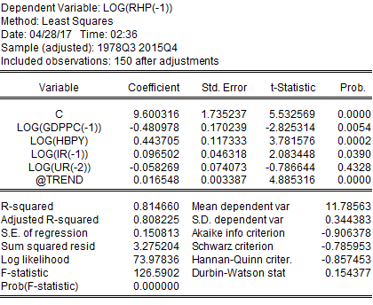
EViews provides the value of Durbin-Watson statistics when a regression in the run. The regression table above showed that Durbin-Watson statistics for this regression were 0.1543, which means that this project soundly rejects the null hypothesis of no serial correlation. If there were no serial correlation, the Durbin-Watson statistics should have been around 2. In this case, the Durbin-Watson statistic falls below two, which indicates a positive serial correlation. On the other hand, the Breusch-Godfrey test for serial correlation indicates that the probability of chi-square is statistically significant. This implies that the regression performed after adjustment for time trend is suffering from serial correlation.
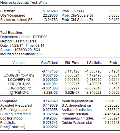
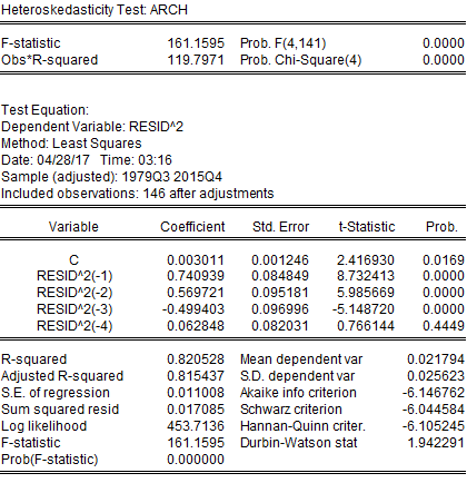
In addition to serial correlation, this project may also suffer from heteroskedasticity because, in many financial and economic time series, the conditional variance of the error term depends on past values of the error term. This may indicate autoregressive conditional heteroskedasticity. However, this project has tested for heteroskedasticity; if this regression did not suffer from heteroskedasticity, the only serial correlation would be corrected. To detect heteroskedasticity, this project has employed the White and ARCH LM tests. Both the White and ARCH LM tests provided similar results where the probability of chi-square was statistically significant. Therefore, this project has found that the regression performed after trend adjustment suffered from both serial correlation and heteroskedasticity. This project needed to adjust standard errors in case of the presence of both serial correlation and heteroskedasticity. Both these issues have been addressed by the HAC (Newey-West) standard errors test. After adjusting for both autocorrelation and heteroskedasticity, it has been found that only HBPY was statistically significant, but the concern for low Durbin-Watson statistics remained (results in Appendix). This implies that even after addressing autocorrelation and heteroskedasticity, the problem of serial correlation remained in the regression model. To solve this issue ARMA model was applied. After applying ARMA model following result has been obtained:
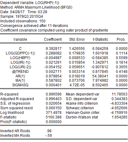
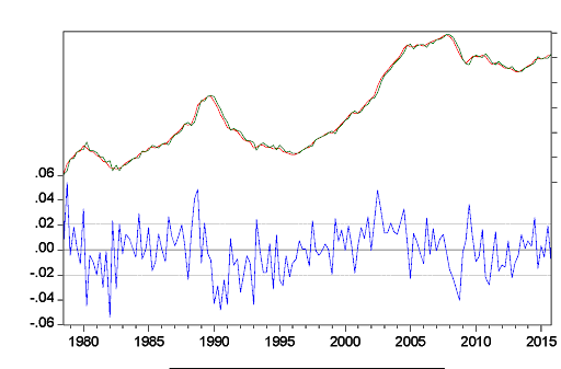
From this regression, it can be seen that neither of the variables exhibits statistical significance, which implies that housing prices do not get affected by these variables rather than other unexplained variables. The Durbin-Watson statistics has also increased to 1.65, which is around 2 indicating reduced serial correlation. The residual plot of this regression (following graph) also indicates moderate behaviour of residuals.
For confirmation of no persistent autocorrelation in this regression, this project has run a higher-order ARMA model, which provides the following result:
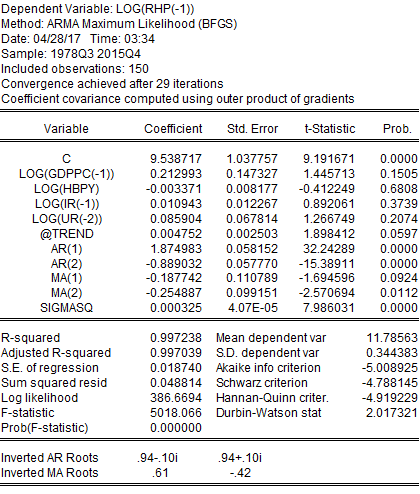
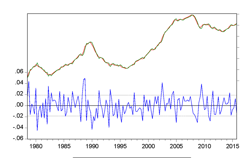
The result clearly demonstrates that this regression has no serial correlation, and residuals are behaving more even. It has finally been found that GDPPC, HBPY, IR, and UR have no statistical influence over RHP. These variables had no statistical significance as well. Based on this regression model, it can be concluded that all the hypotheses have been rejected for this project implying housing prices get affected by another unexplainable variable.
Conclusion
This project has studied the housing prices in the UK considering GDP per capita, interest rate, houses built per year, and the unemployment rate as major determinants. It has been primarily observed that all these variables had a statistically significant impact on housing prices, but this was not true in the end after the regression model had been adjusted for non-stationarity, serial correlation, and heteroskedasticity. Finally, this project has found inconclusive evidence to support the significant impact of GDP per capita, houses built per year, interest rate, and unemployment rate on housing prices in the UK for 1978-2015.
Reference
Attanasio, O. and Weber, G. (2014). The UK Consumption Boom of the Late 1980s: Aggregate Implications of Microeconomic Evidence. The Economic Journal, 104(427), p.1269.
Bełej, M. and Kulesza, S. (2014). The Influence of Financing On The Dynamics Of Housing Prices. Folia Oeconomica Stetinensia, 14(2).
Cheng, A. and Fung, M. (2015). Determinants of Housing Prices. Journal of Economics, Business, and Management, 3(3), pp.352-355.
Cohen, V. and Karpavičiūtė, L. (2017). The analysis of the determinants of housing prices. Independent Journal of Management & Production, 8(1), pp.49-63.
Fiva, J. and Kirkebøen, L. (2011). Information Shocks and the Dynamics of the Housing Market*. Scandinavian Journal of Economics, p.no-no.
HM Treasury (2010). [ARCHIVED CONTENT] UK Government Web Archive – The National Archives. [online] Webarchive.nationalarchives.gov.uk. Available at: http://webarchive.nationalarchives.gov.uk/+/http:/www.hm-treasury.gov.uk/barker_review_of_housing_supply_recommendations.htm [Accessed 27 Apr. 2017].
Meese, R. and Wallace, N. (2014). House Price Dynamics and Market Fundamentals: The Parisian Housing Market. Urban Studies, 40(5-6), pp.1027-1045.
PwC (2017). UK Economic Outlook July 2015: Housing market outlook moderates, but the rise of Generation Rent will continue. [online] PwC. Available at: http://www.pwc.co.uk/services/economics-policy/insights/uk-economic-outlook/ukeo-july2015-housing-market-outlook.html [Accessed 27 Apr. 2017].
Yun Joe Wong, T., Man Eddie Hui, C. and Seabrooke, W. (2013). The impact of interest rates upon housing prices: an empirical study of Hong Kong’s market. Property Management, 21(2), pp.153-170.
Research Log
1st Phase
- Choice of Topic between Housing Prices Determinants or Labour Productivity.
- Finally chosen to study Housing Prices because of data availability and personal interest.
- Selection of variables and collection of secondary data.
- A proposal for the project is submitted.
2nd Phase
- Methods Planner is submitted.
- Assembled secondary data into MS Excel worksheet.
- Met supervisor for further guidelines.
3rd Phase
- Extracted data into EViews workfare from MS Excel worksheet.
- Ran correlation analysis on the variables.
- Ran simple regression on the dataset.
- Unit Root test is performed for stationarity.
- Ordinary Least Square regression is performed.
- Tested the regression for Trend effect.
- Again, OLS is run.
- Tested regression for Autocorrelation and Heteroskedasticity.
- Adjusted for Autocorrelation and Heteroskedasticity.
- Finally, OLS is run after addressing Autocorrelation and Heteroskedasticity.
4th Phase
- Started writing reports based on analyses performed.
- Created reference list and appendix.
- Formatted the report and finalised it for submission.
Appendices
Graph
Correlation
Unit Root Test
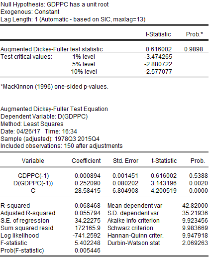
GDPPC has a unit root with t-statistic being lower than all critical values. This clearly demonstrates the non-stationarity characteristic of GDPPC. So we have tested if the first difference of GDPPC has a unit root or not.
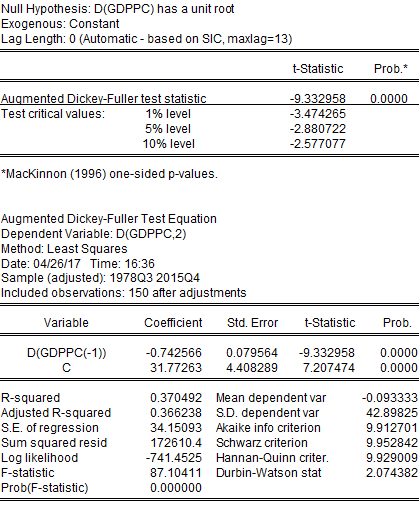
We have found that the first difference of GDPPC has no unit root, with t-statistic being higher than all critical values, implying the first difference of GDPPC is stationary. For this reason, we have used the first difference of GDPPC for further econometric analysis.
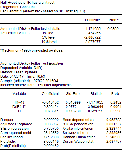
IR is non-stationary.
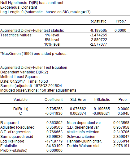
The first difference of IR is stationary.
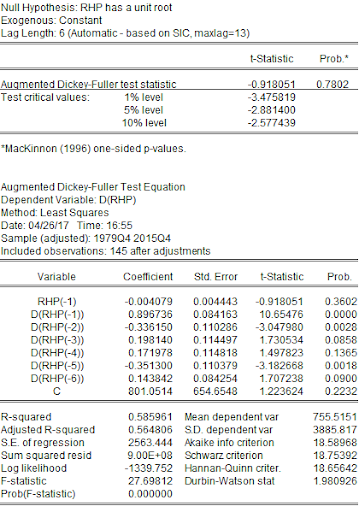
RHP is non-stationary.
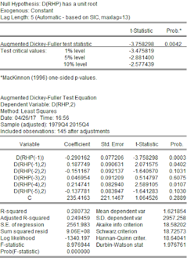
The first difference of RHP is stationary.
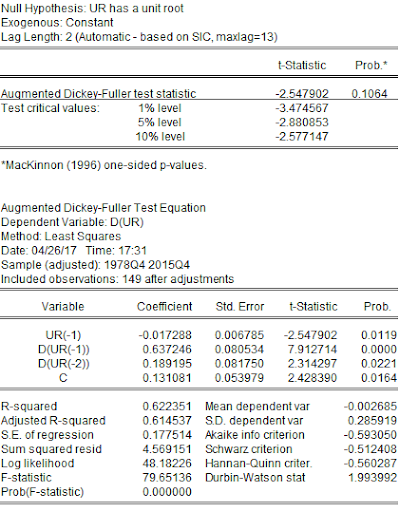
UR is non-stationary.
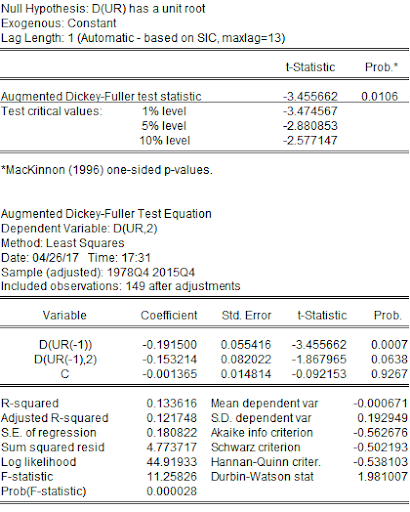
The first difference of UR is also non-stationary.
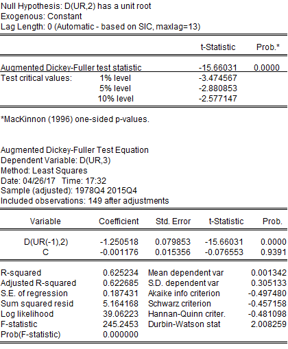
The second difference of UR is stationary.
Autocorrelation and Heteroskedasticity
Heteroskedasticity: White
Heteroskedasticity: ARCH LM
Addressing Autocorrelation and Heteroskedasticity