
An imaginary survey on alcohol consumption among 60 participants is conducted, containing 11 quantitative and qualitative variables. The variables and the variables’ levels are coded and analysed in SPSS and MS Excel 2013 used for graphical representation. This survey was conducted among 30 males and 30 females within middle-aged persons (Mean: 54.04, SD: 12.34). Here researchers check the descriptive statistics of the variables, correlations with alcohol consumption and other quantitative variables are checked, ANOVA is used to check the effect of different regions in alcohol consumption, regression is used to predict the other variables on alcohol consumption. The researcher always considers a 95% confidence interval (0.05 level of significance) for statistical significance, so consider the importance of p-value <0.05 as a convention.
From the beginning of the data, the analysis researcher depicts descriptive statistics (Table1) for the quantitative variable as mean and standard deviation and qualitative variable use median. Here calculating annual income, researchers use median cause income data are usually affected by outlier value. Moreover, the median is also used for ordinal variables like belief, enjoyment, and quality of life.
The researcher also demonstrates a graphical representation of alcohol consumption and the opinion of the respondents on 7 points Likert scale.
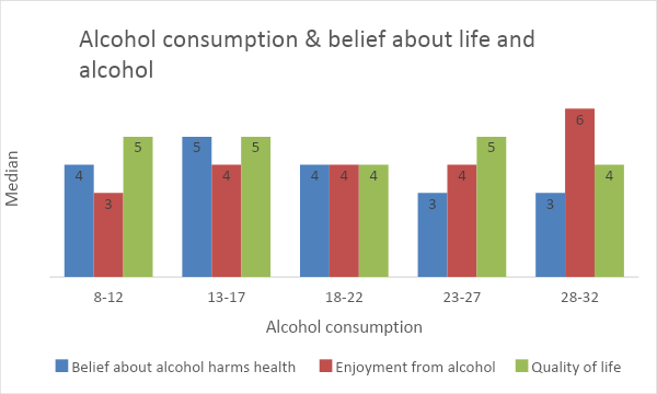
From the above chart, more consumed alcohol got more enjoyment from it, and they are also reluctant that alcohol harms health. All types of alcohol consumption groups think that their quality of life is average or below average.
The researcher calculates correlation(Table 2) among the quantitative variables, so according to SPSS output, the only significant correlation coefficient for average units alcohol per unit and maximum units of one sitting in the past month is .468. There is a moderate positive correlation between intermediate alcohol units and maximum units in the past month. And the rest of the variables don’t have a significant correlation with average alcohol consumption.
The mean of the average alcohol units in the west region is the highest. From the ANOVA table, we get the “sig” value of .029, which is less than P= 0.05. There is a statistically significant difference among the four regions on average alcohol consumption. If we see the pairwise comparison, a significant difference exists between the northeast and north-west region. And there is no significant difference between the north and south regions. There is also a significant correlation between the quality of life and the region r= .03, P=0.01(2-tailed).
Average alcohol consumption may vary from region to region. According to SPSS output (Table 3), there was a statistically significant difference in moderate alcohol consumption among regions by one-way ANOVA (F (3, 56) = 3.23, p = 0.03). So average alcohol consumption in the four areas is different; for further justification, researchers used pairwise comparison (Table 4), which revealed that alcohol consumption of the north-east (p =0.04) and north-west (p = 0.01) regions are statistically significant. So average alcohol in the different areas differs for north-east and north-west region pairs.
The prediction of alcohol consumption from the other significant single values has been performed in SPSS (Table 5). Since R-square tells us the goodness of fit of the model, our R-square for this model is .348, which means that our independent variables can explain 34.8% of the change in average alcohol consumption. Most units in one sitting alcohol consumption in the last month and the highest level of education has statistically significant variables concerning the dependent variable. So, according to the regression coefficient value, one unit increase in one sitting alcohol consumption will increase alcohol consumption in on average 0.28 unit keeping all other variable constant, and more interestingly, one unit increase in education will increase alcohol consumption in one week in on average 1.17 unit keeping all other variables in continuous level.
Appendix:
Table 1: Descriptive statistics of the variables
Quantitative Variables | Mean ± SD | Qualitative variables | Median |
Age | 54.03 ± 12.34 | Belief alcohol harms health (7 point scales) | 4 |
Average alcohol consumption(units/week) | 17 ± 5 | Enjoyment from alcohol (7 point scales) | 4 |
Highest units alcohol consumption in one sitting in last month | 10 ± 7 | Quality of life (7 point scales) | 5 |
Outgoingness | 15 ± 7 | Annual income (in 000s) | 28.50 |
Highest level of education | 3 = University Bachelors (Mode) |
Table 2: Correlations among quantitative variables
Age | Average alcohol units/week | Most units in one sitting in last month | Outgoingness | Annual income in 000s | ||
Age | Pearson Correlation | 1 | -.003 | -.009 | .117 | -.006 |
Sig. (2-tailed) | .981 | .945 | .375 | .961 | ||
N | 60 | 60 | 60 | 60 | 60 | |
Average alc units/week | Pearson Correlation | -.003 | 1 | .468** | -.145 | -.068 |
Sig. (2-tailed) | .981 | .000 | .267 | .604 | ||
N | 60 | 60 | 60 | 60 | 60 | |
Most units in one sitting in last month | Pearson Correlation | -.009 | .468** | 1 | -.208 | -.015 |
Sig. (2-tailed) | .945 | .000 | .111 | .911 | ||
N | 60 | 60 | 60 | 60 | 60 | |
Outgoingness | Pearson Correlation | .117 | -.145 | -.208 | 1 | .218 |
Sig. (2-tailed) | .375 | .267 | .111 | .094 | ||
N | 60 | 60 | 60 | 60 | 60 | |
Annual income in 000s | Pearson Correlation | -.006 | -.068 | -.015 | .218 | 1 |
Sig. (2-tailed) | .961 | .604 | .911 | .094 | ||
N | 60 | 60 | 60 | 60 | 60 | |
**. Correlation is significant at the 0.01 level (2-tailed). | ||||||
Table 3: ANOVA for alcohol consumption in different regions
ANOVA | |||||
Average alcohol consumption units/week | |||||
Sum of Squares | df | Mean Square | F | Sig. | |
Between Groups | 232.183 | 3 | 77.394 | 3.223 | .029 |
Within Groups | 1344.800 | 56 | 24.014 | ||
Total | 1576.983 | 59 | |||
Table 4: Multiple comparisons of different regions
Multiple Comparisons | ||||||
Dependent Variable: Average alcohol consumption units/week | ||||||
LSD | ||||||
(I) Region of country | (J) Region of country | Mean Difference (I-J) | Std. Error | Sig. | 95% Confidence Interval | |
Lower Bound | Upper Bound | |||||
North | South | -1.667 | 1.789 | .356 | -5.25 | 1.92 |
East | -3.800* | 1.789 | .038 | -7.38 | -.22 | |
West | -5.133* | 1.789 | .006 | -8.72 | -1.55 | |
South | North | 1.667 | 1.789 | .356 | -1.92 | 5.25 |
East | -2.133 | 1.789 | .238 | -5.72 | 1.45 | |
West | -3.467 | 1.789 | .058 | -7.05 | .12 | |
East | North | 3.800* | 1.789 | .038 | .22 | 7.38 |
South | 2.133 | 1.789 | .238 | -1.45 | 5.72 | |
West | -1.333 | 1.789 | .459 | -4.92 | 2.25 | |
West | North | 5.133* | 1.789 | .006 | 1.55 | 8.72 |
South | 3.467 | 1.789 | .058 | -.12 | 7.05 | |
East | 1.333 | 1.789 | .459 | -2.25 | 4.92 | |
*. The mean difference is significant at the 0.05 level. | ||||||
Table 5: Regression output on average alcohol consumption
Model | Unstandardised Coefficients | Standardised Coefficients | t | Sig. | 95.0% Confidence Interval for B | |||
B | Std. Error | Beta | Lower Bound | Upper Bound | ||||
1 | (Constant) | 10.156 | 1.978 | 5.135 | .000 | 6.192 | 14.119 | |
Most units in one sitting in last month | .279 | .077 | .404 | 3.639 | .001 | .125 | .432 | |
Sex | 1.986 | 1.136 | .194 | 1.748 | .086 | -.291 | 4.263 | |
Highest level of education | 1.171 | .449 | .287 | 2.604 | .012 | .270 | 2.071 | |
Annual income in 000s | -.009 | .031 | -.031 | -.282 | .779 | -.070 | .053 | |
a. Dependent Variable: Average alcohol units/week | ||||||||